


ASTM E739-10(2015)
(Practice)Standard Practice for Statistical Analysis of Linear or Linearized Stress-Life (S-N) and Strain-Life (ε-N) Fatigue Data
Standard Practice for Statistical Analysis of Linear or Linearized Stress-Life (<emph type="bdit">S-N</emph>) and Strain-Life (ε-<emph type="bdit" >N</emph>) Fatigue Data
SIGNIFICANCE AND USE
4.1 Materials scientists and engineers are making increased use of statistical analyses in interpreting S-N and ε-N fatigue data. Statistical analysis applies when the given data can be reasonably assumed to be a random sample of (or representation of) some specific defined population or universe of material of interest (under specific test conditions), and it is desired either to characterize the material or to predict the performance of future random samples of the material (under similar test conditions), or both.
SCOPE
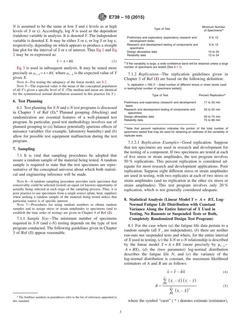
1.1 This practice covers only S-N and ε-N relationships that may be reasonably approximated by a straight line (on appropriate coordinates) for a specific interval of stress or strain. It presents elementary procedures that presently reflect good practice in modeling and analysis. However, because the actual S-N or ε-N relationship is approximated by a straight line only within a specific interval of stress or strain, and because the actual fatigue life distribution is unknown, it is not recommended that (a) the S-N or ε-N curve be extrapolated outside the interval of testing, or (b) the fatigue life at a specific stress or strain amplitude be estimated below approximately the fifth percentile (P ≃ 0.05). As alternative fatigue models and statistical analyses are continually being developed, later revisions of this practice may subsequently present analyses that permit more complete interpretation of S-N and ε-N data.
General Information
Buy Standard
Standards Content (Sample)
NOTICE: This standard has either been superseded and replaced by a new version or withdrawn.
Contact ASTM International (www.astm.org) for the latest information
Designation: E739 − 10 (Reapproved 2015)
Standard Practice for
Statistical Analysis of Linear or Linearized Stress-Life (S-N)
and Strain-Life (ε-N) Fatigue Data
This standard is issued under the fixed designation E739; the number immediately following the designation indicates the year of
original adoption or, in the case of revision, the year of last revision. A number in parentheses indicates the year of last reapproval. A
superscript epsilon (´) indicates an editorial change since the last revision or reapproval.
1. Scope 3. Terminology
3.1 The terms used in this practice shall be used as defined
1.1 This practice covers only S-N and ε-N relationships that
in Definitions E206 and E513. In addition, the following
may be reasonably approximated by a straight line (on appro-
terminology is used:
priate coordinates) for a specific interval of stress or strain. It
3.1.1 dependent variable—the fatigue life N (or the loga-
presents elementary procedures that presently reflect good
rithm of the fatigue life).
practice in modeling and analysis. However, because the actual
3.1.1.1 Discussion—Log (N) is denoted Y in this practice.
S-N or ε-N relationship is approximated by a straight line only
3.1.2 independent variable—the selected and controlled
within a specific interval of stress or strain, and because the
variable (namely, stress or strain). It is denoted X in this
actual fatigue life distribution is unknown, it is not recom-
practice when plotted on appropriate coordinates.
mended that (a) the S-N or ε-N curve be extrapolated outside
3.1.3 log-normal distribution—the distribution of N when
the interval of testing, or (b) the fatigue life at a specific stress
log (N) is normally distributed. (Accordingly, it is convenient
or strain amplitude be estimated below approximately the fifth
to analyze log (N) using methods based on the normal
percentile (P . 0.05). As alternative fatigue models and
distribution.)
statistical analyses are continually being developed, later
3.1.4 replicate (repeat) tests—nominally identical tests on
revisions of this practice may subsequently present analyses
different randomly selected test specimens conducted at the
that permit more complete interpretation of S-N and ε-N data.
same nominal value of the independent variable X. Such
replicate or repeat tests should be conducted independently; for
2. Referenced Documents
example, each replicate test should involve a separate set of the
test machine and its settings.
2.1 ASTM Standards:
3.1.5 run out—no failure at a specified number of load
E206 Definitions of Terms Relating to Fatigue Testing and
cycles (Practice E468).
the Statistical Analysis of Fatigue Data; Replaced by
3.1.5.1 Discussion—The analyses illustrated in this practice
E 1150 (Withdrawn 1988)
do not apply when the data include either run-outs (or
E468 Practice for Presentation of Constant Amplitude Fa-
suspended tests). Moreover, the straight-line approximation of
tigue Test Results for Metallic Materials
the S-N or ε-N relationship may not be appropriate at long lives
E513 Definitions of Terms Relating to Constant-Amplitude,
when run-outs are likely.
Low-Cycle Fatigue Testing; Replaced by E 1150 (With-
3 3.1.5.2 Discussion—For purposes of statistical analysis, a
drawn 1988)
run-out may be viewed as a test specimen that has either been
E606/E606M Test Method for Strain-Controlled Fatigue
removed from the test or is still running at the time of the data
Testing
analysis.
4. Significance and Use
This practice is under the jurisdiction of ASTM Committee E08 on Fatigue and
4.1 Materials scientists and engineers are making increased
Fracture and is the direct responsibility of Subcommittee E08.04 on Structural
Applications. use of statistical analyses in interpreting S-N and ε-N fatigue
Current edition approved Oct. 1, 2015. Published November 2015. Originally
data. Statistical analysis applies when the given data can be
approved in 1980. Last previous edition approved in 2010 as E739 – 10. DOI:
reasonably assumed to be a random sample of (or representa-
10.1520/E0739-10R15.
tion of) some specific defined population or universe of
For referenced ASTM standards, visit the ASTM website, www.astm.org, or
contact ASTM Customer Service at service@astm.org. For Annual Book of ASTM
material of interest (under specific test conditions), and it is
Standards volume information, refer to the standard’s Document Summary page on
desired either to characterize the material or to predict the
the ASTM website.
3 performance of future random samples of the material (under
The last approved version of this historical standard is referenced on www.ast-
m.org. similar test conditions), or both.
Copyright © ASTM International, 100 Barr Harbor Drive, PO Box C700, West Conshohocken, PA 19428-2959. United States
E739 − 10 (2015)
5. Types of S-N and ε-N Curves Considered 5.1.1 The fatigue life N is the dependent (random) variable
in S-N and ε-N tests, whereas S or ε is the independent
5.1 It is well known that the shape of S-N and ε-N curves
(controlled) variable.
can depend markedly on the material and test conditions. This
practice is restricted to linear or linearized S-N and ε-N
NOTE 2—In certain cases, the independent variable used in analysis is
relationships, for example,
not literally the variable controlled during testing. For example, it is
common practice to analyze low-cycle fatigue data treating the range of
log N 5 A1B ~S! or (1)
plastic strain as the controlled variable, when in fact the range of total
strain was actually controlled during testing. Although there may be some
log N 5 A1B ~ε! or
question regarding the exact nature of the controlled variable in certain
log N 5 A1B logS or (2) S-N and ε-N tests, there is never any doubt that the fatigue life is the
~ !
dependent variable.
log N 5 A1B logε
~ !
NOTE 3—In plotting S-N and ε-N curves, the independent variables S
in which S and ε may refer to (a) the maximum value of
and ε are plotted along the ordinate, with life (the dependent variable)
constant-amplitude cyclic stress or strain, given a specific
plotted along the abscissa. Refer, for example, to Fig. 1.
value of the stress or strain ratio, or of the minimum cyclic
5.1.2 The distribution of fatigue life (in any test) is unknown
stress or strain, (b) the amplitude or the range of the
(and indeed may be quite complex in certain situations). For
constant-amplitude cyclic stress or strain, given a specific
value of the mean stress or strain, or (c) analogous informa- the purposes of simplifying the analysis (while maintaining
tion stated in terms of some appropriate independent (con-
sound statistical procedures), it is assumed in this practice that
trolled) variable.
the logarithms of the fatigue lives are normally distributed, that
NOTE 1—In certain cases, the amplitude of the stress or strain is not
is, the fatigue life is log-normally distributed, and that the
constant during the entire test for a given specimen. In such cases some
variance of log life is constant over the entire range of the
effective (equivalent) value of S or ε must be established for use in
analysis. independent variable used in testing (that is, the scatter in log
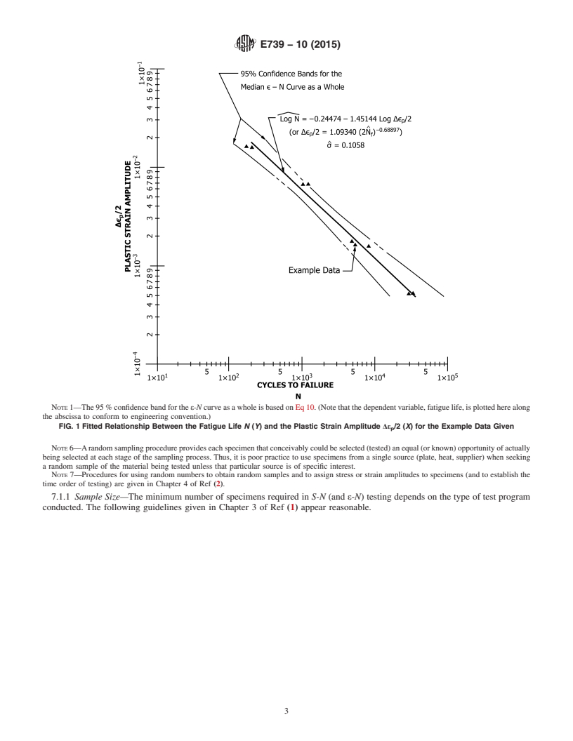
NOTE 1—The 95 % confidence band for the ε-N curve as a whole is based on Eq 10. (Note that the dependent variable, fatigue life, is plotted here along
the abscissa to conform to engineering convention.)
FIG. 1 Fitted Relationship Between the Fatigue Life N (Y) and the Plastic Strain Amplitude Δε /2 (X) for the Example Data Given
p
E739 − 10 (2015)
N is assumed to be the same at low S and ε levels as at high
Minimum Number
Type of Test
A
of Specimens
levels of S or ε). Accordingly, log N is used as the dependent
(random) variable in analysis. It is denoted Y. The independent
Preliminary and exploratory (exploratory research and 6 to 12
variable is denoted X. It may be either S or ε, or log S or log ε,
development tests)
Research and development testing of components and 6 to 12
respectively, depending on which appears to produce a straight
specimens
line plot for the interval of S or ε of interest. Thus Eq 1 and Eq
Design allowables data 12 to 24
2 may be re-expressed as Reliability data 12 to 24
Y 5 A1BX (3)
A
If the variability is large, a wide confidence band will be obtained unless a large
number of specimens are tested (See 8.1.1).
Eq 3 is used in subsequent analysis. It may be stated more
precisely as µ 5A1BX, where µ is the expected value of Y
Y ? X Y ? X
7.1.2 Replication—The replication guidelines given in
given X.
Chapter 3 of Ref (1) are based on the following definition:
NOTE 4—For testing the adequacy of the linear model, see 8.2.
% replication = 100 [1 − (total number of different stress or strain levels used
NOTE 5—The expected value is the mean of the conceptual population
in testing/total number of specimens tested)]
of all Y’s given a specific level of X. (The median and mean are identical
for the symmetrical normal distribution assumed in this practice for Y.) A
Type of Test Percent Replication
6. Test Planning
Preliminary and exploratory (research and development 17 to 33 min
tests)
6.1 Test planning for S-N and ε-N test programs is discussed
Research and development testing of components and 33 to 50 min
in Chapter 3 of Ref (1). Planned grouping (blocking) and
specimens
Design allowables data 50 to 75 min
randomization are essential features of a well-planned test
Reliability data 75 to 88 min
program. In particular, good test methodology involves use of
planned grouping to (a) balance potentially spurious effects of A
Note that percent replication indicates the portion of the total number of
nuisance variables (for example, laboratory humidity) and (b)
specimens tested that may be used for obtaining an estimate of the variability of
replicate tests.
allow for possible test equipment malfunction during the test
program.
7.1.2.1 Replication Examples—Good replication: Suppose
that ten specimens are used in research and development for
7. Sampling
the testing of a component. If two specimens are tested at each
7.1 It is vital that sampling procedures be adopted that
of five stress or strain amplitudes, the test program involves
assure a random sample of the material being tested. A random
50 % replications. This percent replication is considered ad-
sample is required to state that the test specimens are repre-
equate for most research and development applications. Poor
sentative of the conceptual universe about which both statisti-
replication: Suppose eight different stress or strain amplitudes
cal and engineering inference will be made.
are used in testing, with two replicates at each of two stress or
strain amplitudes (and no replication at the other six stress or
NOTE 6—A random sampling procedure provides each specimen that
conceivably could be selected (tested) an equal (or known) opportunity of strain amplitudes). This test program involves only 20 %
actually being selected at each stage of the sampling process. Thus, it is
replication, which is not generally considered adequate.
poor practice to use specimens from a single source (plate, heat, supplier)
when seeking a random sample of the material being tested unless that
8. Statistical Analysis (Linear Model Y = A + BX, Log-
particular source is of specific interest.
NOTE 7—Procedures for using random numbers to obtain random Normal Fatigue Life Distribution with Constant
samples and to assign stress or strain amplitudes to specimens (and to
Variance Along the Entire Interval of X Used in
establish the time order of testing) are given in Chapter 4 of Ref (2).
Testing, No Runouts or Suspended Tests or Both,
7.1.1 Sample Size—The minimum number of specimens Completely Randomized Design Test Program)
required in S-N (and ε-N) testing depends on the type of test
8.1 For the case where (a) the fatigue life data pertain to a
program conducted. The following guidelines given in Chapter
random sample (all Y are independent), (b) there are neither
i
3 of Ref (1) appear reasonable.
run-outs nor suspended tests and where, for the entire interval
of X used in testing, (c) the S-N or ε-N relationship is described
by the linear model Y = A + BX (more precisely by µ 5
Y ? X
A + BX), (d) the (two parameter) log-normal distribution
describes the fatigue life N, and (e) the variance of the
log-normal distribution is constant, the maximum likelihood
estimators of A and B are as follows:
ˆ ¯ ˆ ¯
A 5 Y 2 BX (4)
k
¯ ¯
~X 2 X! ~Y 2 Y!
( i i
i51
ˆ
B 5 (5)
k
¯
~X 2 X!
( i
i51
The boldface numbers in parentheses refer to the list of references appended to
this standard. where the symbol “caret” ( ^ ) denotes estimate (estimator),
E739 − 10 (2015)
–
¯
dence interval. This table has one entry parameter (the statis-
the symbol “overbar” ( ) denotes average (for example, Y
k k
tical degrees of freedom, n, for t ). For Eq 7 and Eq 8, n =
¯
5 Y /k and X5 X /k), Y = log N , X = S or ε , or log S or
( i ( i i i i i i i
k − 2.
i51 i51
log ε (refer to Eq 1 and Eq 2), and k is the total number of test
NOTE 9—The confidence intervals for A and B are exact if conditions
i
(a) through (e) in 8.1 are met exactly. However, these intervals are still
specimens (the total sample size). The recommended expres-
reasonably accurate when the actual life distribution differs slightly from
sion for estimating the variance of the normal distribution for
the (two-parameter) log-normal distribution, that is, when only condition
log N is
(d) is not met exactly, due to the robustness of the t statistic.
k
2 NOTE 10—Because the actual median S-N or ε-N relationship is only
ˆ
~Y 2 Y !
( i i
approximated by a straight line within a specific interval of stress or strain,
i51
σˆ 5 (6)
confidence intervals for A and B that pertain to confidence levels greater
k 2 2
than approximately 0.95 are not recommended.
ˆ
in which Ŷ = Â + BX and the (k − 2) term in the denomi-
i i
2 8.1.1.1 The meaning of the confidence interval associated
nator is used instead of k to make σˆ an unbiased estimator of
2 with, say, Eq 8 is as follows (Note 11). If the values of t given
p
the normal population variance σˆ .
in Table 1 for, say, P = 95 % are used in a series of analyses
NOTE 8—An assumption of constant variance is usually reasonable for
involving the estimation of B from independent data sets, then
notched and joint specimens up to about 10 cycles to failure. The variance
in the long run we may expect 95 % of the computed intervals
of unnotched specimens generally increases with decreasing stress (strain)
to include the value B. If in each instance we were to assert that
level (see Section
...
This document is not an ASTM standard and is intended only to provide the user of an ASTM standard an indication of what changes have been made to the previous version. Because
it may not be technically possible to adequately depict all changes accurately, ASTM recommends that users consult prior editions as appropriate. In all cases only the current version
of the standard as published by ASTM is to be considered the official document.
Designation: E739 − 10 E739 − 10 (Reapproved 2015)
Standard Practice for
Statistical Analysis of Linear or Linearized Stress-Life (S-N)
and Strain-Life (ε-N) Fatigue Data
This standard is issued under the fixed designation E739; the number immediately following the designation indicates the year of
original adoption or, in the case of revision, the year of last revision. A number in parentheses indicates the year of last reapproval. A
superscript epsilon (´) indicates an editorial change since the last revision or reapproval.
1. Scope
1.1 This practice covers only S-N and ε-N relationships that may be reasonably approximated by a straight line (on appropriate
coordinates) for a specific interval of stress or strain. It presents elementary procedures that presently reflect good practice in
modeling and analysis. However, because the actual S-N or ε-N relationship is approximated by a straight line only within a specific
interval of stress or strain, and because the actual fatigue life distribution is unknown, it is not recommended that (a) the S-N or
ε-N curve be extrapolated outside the interval of testing, or (b) the fatigue life at a specific stress or strain amplitude be estimated
below approximately the fifth percentile (P . 0.05). As alternative fatigue models and statistical analyses are continually being
developed, later revisions of this practice may subsequently present analyses that permit more complete interpretation of S-N and
ε-N data.
2. Referenced Documents
2.1 ASTM Standards:
E206 Definitions of Terms Relating to Fatigue Testing and the Statistical Analysis of Fatigue Data; Replaced by E 1150
(Withdrawn 1988)
E468 Practice for Presentation of Constant Amplitude Fatigue Test Results for Metallic Materials
E513 Definitions of Terms Relating to Constant-Amplitude, Low-Cycle Fatigue Testing; Replaced by E 1150 (Withdrawn
1988)
E606E606/E606M Test Method for Strain-Controlled Fatigue Testing
3. Terminology
3.1 The terms used in this practice shall be used as defined in Definitions E206 and E513. In addition, the following terminology
is used:
3.1.1 dependent variable—the fatigue life N (or the logarithm of the fatigue life).
3.1.1.1 Discussion—Log (N) is denoted Y in this practice.
3.1.2 independent variable—the selected and controlled variable (namely, stress or strain). It is denoted X in this practice when
plotted on appropriate coordinates.
3.1.3 log-normal distribution—the distribution of N when log (N) is normally distributed. (Accordingly, it is convenient to
analyze log (N) using methods based on the normal distribution.)
3.1.4 replicate (repeat) tests—nominally identical tests on different randomly selected test specimens conducted at the same
nominal value of the independent variable X. Such replicate or repeat tests should be conducted independently; for example, each
replicate test should involve a separate set of the test machine and its settings.
3.1.5 run out—no failure at a specified number of load cycles (Practice E468).
3.1.5.1 Discussion—The analyses illustrated in this practice do not apply when the data include either run-outs (or suspended
tests). Moreover, the straight-line approximation of the S-N or ε-N relationship may not be appropriate at long lives when run-outs
are likely.
This practice is under the jurisdiction of ASTM Committee E08 on Fatigue and Fracture and is the direct responsibility of Subcommittee E08.04 on Structural
Applications.
Current edition approved Nov. 1, 2010Oct. 1, 2015. Published November 2010November 2015. Originally approved in 1980. Last previous edition approved in 20042010
ε1
as E739 – 91 (2004)E739 – 10. . DOI: 10.1520/E0739-10.10.1520/E0739-10R15.
For referenced ASTM standards, visit the ASTM website, www.astm.org, or contact ASTM Customer Service at service@astm.org. For Annual Book of ASTM Standards
volume information, refer to the standard’s Document Summary page on the ASTM website.
The last approved version of this historical standard is referenced on www.astm.org.
Copyright © ASTM International, 100 Barr Harbor Drive, PO Box C700, West Conshohocken, PA 19428-2959. United States
E739 − 10 (2015)
3.1.5.2 Discussion—For purposes of statistical analysis, a run-out may be viewed as a test specimen that has either been
removed from the test or is still running at the time of the data analysis.
4. Significance and Use
4.1 Materials scientists and engineers are making increased use of statistical analyses in interpreting S-N and ε-N fatigue data.
Statistical analysis applies when the given data can be reasonably assumed to be a random sample of (or representation of) some
specific defined population or universe of material of interest (under specific test conditions), and it is desired either to characterize
the material or to predict the performance of future random samples of the material (under similar test conditions), or both.
5. Types of S-N and ε-N Curves Considered
5.1 It is well known that the shape of S-N and ε-N curves can depend markedly on the material and test conditions. This practice
is restricted to linear or linearized S-N and ε-N relationships, for example,
log N 5 A1B ~S! or (1)
log N 5 A1B ~ε! or
log N 5 A1B logS or (2)
~ !
log N 5 A1B logε
~ !
in which S and ε may refer to (a) the maximum value of constant-amplitude cyclic stress or strain, given a specific value of
the stress or strain ratio, or of the minimum cyclic stress or strain, (b) the amplitude or the range of the constant-amplitude
cyclic stress or strain, given a specific value of the mean stress or strain, or (c) analogous information stated in terms of some
appropriate independent (controlled) variable.
NOTE 1—In certain cases, the amplitude of the stress or strain is not constant during the entire test for a given specimen. In such cases some effective
(equivalent) value of S or ε must be established for use in analysis.
5.1.1 The fatigue life N is the dependent (random) variable in S-N and ε-N tests, whereas S or ε is the independent (controlled)
variable.
NOTE 2—In certain cases, the independent variable used in analysis is not literally the variable controlled during testing. For example, it is common
practice to analyze low-cycle fatigue data treating the range of plastic strain as the controlled variable, when in fact the range of total strain was actually
controlled during testing. Although there may be some question regarding the exact nature of the controlled variable in certain S-N and ε-N tests, there
is never any doubt that the fatigue life is the dependent variable.
NOTE 3—In plotting S-N and ε-N curves, the independent variables S and ε are plotted along the ordinate, with life (the dependent variable) plotted
along the abscissa. Refer, for example, to Fig. 1.
5.1.2 The distribution of fatigue life (in any test) is unknown (and indeed may be quite complex in certain situations). For the
purposes of simplifying the analysis (while maintaining sound statistical procedures), it is assumed in this practice that the
logarithms of the fatigue lives are normally distributed, that is, the fatigue life is log-normally distributed, and that the variance
of log life is constant over the entire range of the independent variable used in testing (that is, the scatter in log N is assumed to
be the same at low S and ε levels as at high levels of S or ε). Accordingly, log N is used as the dependent (random) variable in
analysis. It is denoted Y. The independent variable is denoted X. It may be either S or ε, or log S or log ε, respectively, depending
on which appears to produce a straight line plot for the interval of S or ε of interest. Thus Eq 1 and Eq 2 may be re-expressed as
Y 5 A1BX (3)
Eq 3 is used in subsequent analysis. It may be stated more precisely as μ 5A1BX, where μ is the expected value of Y given
Y ? X Y ? X
X.
NOTE 4—For testing the adequacy of the linear model, see 8.2.
NOTE 5—The expected value is the mean of the conceptual population of all Y’s given a specific level of X. (The median and mean are identical for
the symmetrical normal distribution assumed in this practice for Y.)
6. Test Planning
6.1 Test planning for S-N and ε-N test programs is discussed in Chapter 3 of Ref (1). Planned grouping (blocking) and
randomization are essential features of a well-planned test program. In particular, good test methodology involves use of planned
grouping to (a) balance potentially spurious effects of nuisance variables (for example, laboratory humidity) and (b) allow for
possible test equipment malfunction during the test program.
7. Sampling
7.1 It is vital that sampling procedures be adopted that assure a random sample of the material being tested. A random sample
is required to state that the test specimens are representative of the conceptual universe about which both statistical and engineering
inference will be made.
The boldface numbers in parentheses refer to the list of references appended to this standard.
E739 − 10 (2015)
NOTE 1—The 95 % confidence band for the ε-N curve as a whole is based on Eq 10. (Note that the dependent variable, fatigue life, is plotted here along
the abscissa to conform to engineering convention.)
FIG. 1 Fitted Relationship Between the Fatigue Life N (Y) and the Plastic Strain Amplitude Δε /2 (X) for the Example Data Given
p
NOTE 6—A random sampling procedure provides each specimen that conceivably could be selected (tested) an equal (or known) opportunity of actually
being selected at each stage of the sampling process. Thus, it is poor practice to use specimens from a single source (plate, heat, supplier) when seeking
a random sample of the material being tested unless that particular source is of specific interest.
NOTE 7—Procedures for using random numbers to obtain random samples and to assign stress or strain amplitudes to specimens (and to establish the
time order of testing) are given in Chapter 4 of Ref (2).
7.1.1 Sample Size—The minimum number of specimens required in S-N (and ε-N) testing depends on the type of test program
conducted. The following guidelines given in Chapter 3 of Ref (1) appear reasonable.
E739 − 10 (2015)
Minimum Number
Type of Test
A
of Specimens
Preliminary and exploratory (exploratory research and 6 to 12
development tests)
Research and development testing of components and 6 to 12
specimens
Design allowables data 12 to 24
Reliability data 12 to 24
A
If the variability is large, a wide confidence band will be obtained unless a large number of specimens are tested (See 8.1.1).
7.1.2 Replication—The replication guidelines given in Chapter 3 of Ref (1) are based on the following definition:
% replication = 100 [1 − (total number of different stress or strain levels used in testing/total number of specimens
tested)]
A
Type of Test Percent Replication
Preliminary and exploratory (research and development 17 to 33 min
tests)
Research and development testing of components and 33 to 50 min
specimens
Design allowables data 50 to 75 min
Reliability data 75 to 88 min
A
Note that percent replication indicates the portion of the total number of specimens tested that may be used for obtaining an estimate of the variability of replicate tests.
7.1.2.1 Replication Examples—Good replication: Suppose that ten specimens are used in research and development for the
testing of a component. If two specimens are tested at each of five stress or strain amplitudes, the test program involves 50 %
replications. This percent replication is considered adequate for most research and development applications. Poor replication:
Suppose eight different stress or strain amplitudes are used in testing, with two replicates at each of two stress or strain amplitudes
(and no replication at the other six stress or strain amplitudes). This test program involves only 20 % replication, which is not
generally considered adequate.
8. Statistical Analysis (Linear Model Y = A + BX, Log-Normal Fatigue Life Distribution with Constant Variance Along
the Entire Interval ofX Used in Testing, No Runouts or Suspended Tests or Both, Completely Randomized Design
Test Program)
8.1 For the case where (a) the fatigue life data pertain to a random sample (all Y are independent), (b) there are neither run-outs
i
nor suspended tests and where, for the entire interval of X used in testing, (c) the S-N or ε-N relationship is described by the linear
model Y = A + BX (more precisely by μ 5 A + BX), (d) the (two parameter) log-normal distribution describes the fatigue life
Y ? X
N, and (e) the variance of the log-normal distribution is constant, the maximum likelihood estimators of A and B are as follows:
ˆ ¯ ˆ ¯
A 5 Y 2 BX (4)
k
¯ ¯
~ ! ~ !
X 2 X Y 2 Y
( i i
i51
ˆ
B 5 (5)
k
¯
~X 2 X!
( i
i51
k
–
¯
where the symbol “caret” ( ^ ) denotes estimate (estimator), the symbol “overbar” ( ) denotes average (for example, Y5 Y /k
(
i
i51
k
¯
and X5 X /k), Y = log N , X = S or ε , or log S or log ε (refer to Eq 1 and Eq 2), and k is the total number of test specimens
(
i i i i i i i i
i51
(the total sample size). The recommended expression for estimating the variance of the normal distribution for log N is
k
ˆ
~Y 2 Y !
( i i
i51
σˆ 5 (6)
k 2 2
in which Ŷ = Â + BˆX and the (k − 2) term in the denominator is used instead of k to make σˆ an unbiased estimator of the
i i
normal population variance σ ˆ .
NOTE 8—An assumption of constant variance is usually reasonable for notched and joint specimens up to about 10 cycles to failure. The variance of
unnotched specimens generally increases with decreasing stress (strain) level (see Section 9). If the assumption of constant variance appears to be dubious,
the reader is referred to Ref (3) for the appropriate statistical test.
8.1.1 Confidence Intervals for Parameters A and B—The estimators  and Bˆ are normally distributed with expected values A
and B, respectively, (regardless of total sample size k) when conditions (a) through (e) in 8.1 are met. Accordingly, confidence
intervals for parameters A and B can be established using the t distribution, Table 1. The confidence interval for A is given by Â
6 t σˆ , or
p Â
E739 − 10 (2015)
TABLE 1 Values of t (Abstracted from STP 313 (4))
p
B
P, %
A
n
90 95
4 2.1318 2.7764
5 2.0150 2.5706
6 1.9432 2.4469
7 1.8946 2.3646
8 1.8595 2.3060
9 1.8331 2.2622
10 1.8125 2.2281
11 1.7959 2.2010
12 1.7823 2.1788
...
Questions, Comments and Discussion
Ask us and Technical Secretary will try to provide an answer. You can facilitate discussion about the standard in here.